
Sperry Lab Methods & Computer Programs
Measuring hydraulic conductivity
Soil-Plant Water Transport Model
Photosynthetic Gain and Hydraulic Cost Optimization Model
Measuring hydraulic conductivity
We use several methods for measuring hydraulic conductivity. The most basic is used for single unbranched stem segments (see graphic below). The stem is attached to solution-filled tubing. We use 20mM KCl mixed in filtered (0.2 µm) water that is purified by passing through deionizing and organic removal cartridges. A KCl solution is used to control for possible ionic effects on pit membrane conductance [however, it is important to rinse and sterilize the tubing periodically with a 10 or 20% Clorox solution]. Using the bypass, we equilibrate the pressure across the stem and measure the "background" flow rate in the absence of an applied pressure. Then, we measure the pressurized flow by switching the upstream stem to the elevated IV bag. This induces a hydraulic head of several kPa depending on the height difference. For big-vesseled material, we use heads of 2 kPa or less to avoid displacing embolisms from open vessels. Otherwise typical heads are 6-7 kPa. Following the pressurized reading, we repeat the background reading. We subtract the average background flow from the pressurized flow to get the net flow rate induced by pressure. This net flow rate is divided by the pressure gradient along the stem to obtain the hydraulic conductivity. We have written an Excel Macro that reads the balance and outputs flow rates and conductivities into the Excel spreadsheet. Click the links to download a copy of this program and instructions ("conduct.ver1.xls" and "balance interface program instructions.doc"). You will also need to add the activex control XMCommCRC.ocx to your Excel to run the program ("XMComm.CRC.ocx").
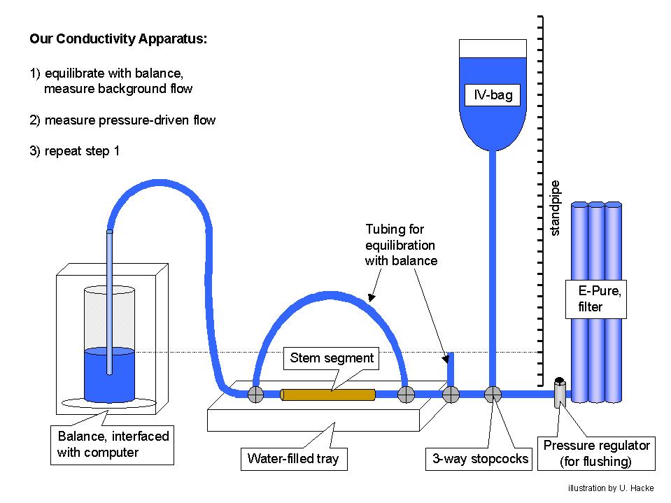
Some recent observations have suggested that an even better way to measure the stem conductivity is to determine the slope of the flow vs. pressure relationship. This is assumed to be perfectly linear in our current calculation. But there may be some non-linearity in the region of the zero pressure intercept. So, we will probably begin to use a set of 3-4 pressure/flow readings to get the conductivity from the slope without having to read the background flow.
In addition to this basic technique, we measure whole-shoot and whole-root system conductivities using a vacuum chamber method (Kolb et al. 1996, PDF). This is useful for measurements of low-conductivity material like leaves, petioles, minor branches, and small roots. We will soon have a version of the Excel conductivity program ready for using with this alternative method.
Vulnerability curves
Over the years we've used many methods to obtain "vulnerability curves" which show the decrease in hydraulic conductivity (or increase in percentage loss of conductivity, PLC) with increasingly negative xylem pressure. Conductivity falls as cavitation knocks out more and more conduits, so this curve tells us how vulnerable the xylem is to cavitation (see graph).
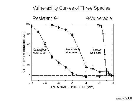
Range of vulnerability curves from resistant (Ceanothus) to vulnerable (Populus).
In order of development, some of the methods:
1. The dehydration method.
This is the original technique (Sperry 1986, PDF), and in some ways may be the most free of artifact. Plants or large branches are dehydrated to measured water potentials—either through natural drought or forced dehydration. Parts, usually stems, are cut from the intact plant underwater and the conductivity is measured. Conductivities can be standardized by dividing them by the cross-sectional area of the stem. These conductivities can be plotted directly vs. water potential to obtain the vulnerability curve. Often, however, the stems are flushed after the initial conductivity measurement to obtain a maximum conductivity and the PLC (percentage loss conductivity) is plotted. However, we've come to prefer using absolute conductivity per stem area rather than PLC because it provides more information.
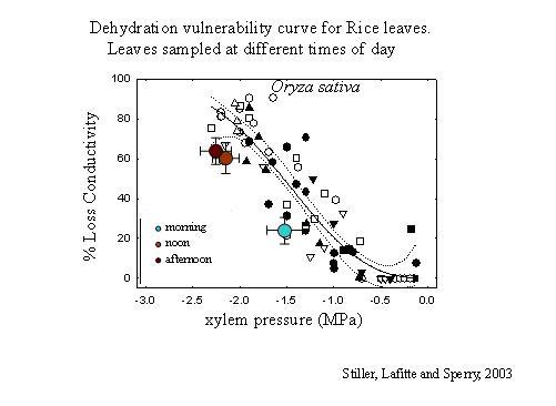
A dehydration vulnerability curve for rice leaves sampled at different times of day.
2. Air-injection method
In this technique (Sperry and Saliendra 1994, PDF), a stem is placed through a double-ended pressure chamber (picture). The conductivity is measured, usually by applying a hydraulic head and collecting water in tared vials of cotton wool. The air pressure is raised and held for 10-15 minutes, then released, and the conductivity is measured again. The procedure is repeated at increasingly greater pressure until the conductivity has dropped to near zero. What is happening is the air is being forced into the vascular system via air-seeding, gradually emptying all of the xylem conduits. The technique generally agrees with dehydration or centrifuge curves (see graph), which is some of the strongest evidence that air-seeding is responsible for cavitation. Plans are available for the machining of these double-ended chambers. Split chambers can be used to induce embolism in intact plants. Other variants on the technique have been used (e.g., Sperry and Tyree 1990, PDF).
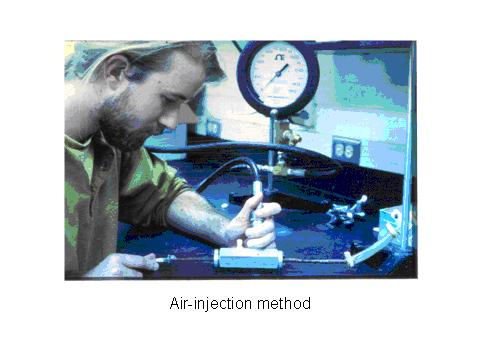
Ex-undergrad Nathan Alder using the double-ended pressure chamber
for measuring air-injection vulnerability curves.
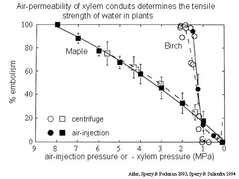
Air-injection curves (solid lines, symbols) generally agree well with centrifuge curves
(dashed lines, open symbols), suggesting that air-seeding is causing cavitation in the xylem.
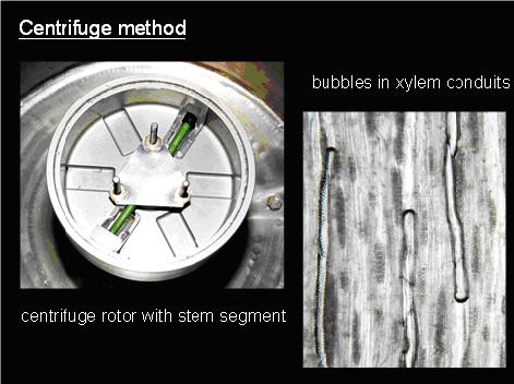
3. Centrifuge methods
The oldest centrifuge method is the so-called "static" method developed by Will Pockman when he was a graduate student in the lab (Pockman et al. 1995, PDF, ; Alder et al. 1997, PDF). Stems or roots are mounted in a custom-built rotor, and spun to generate a negative pressure. The hydraulic conductivity is measured between spinning by removing the stems and measuring them on the tubing apparatus described under "hydraulic conductivity" measurements. Rotors of two sizes (to fit 14 and 27 cm long stems) can be built by the University of Utah Chemistry Department machine shop. These rotors fit Sorvall RC5C or RC5B centrifuges, which are fairly common floor-model centrifuges. Here you can download the drawings for constructing the rotor and reservoirs at a machine shop with US standards and imperial units (Original_Rotor_Design.pdf) or metric system (Rotor_design.pdf).
Herve Cochard has since developed what we call the "flow-centrifuge" method, and we have modified our original rotors so that we can also use his method. In this technique, the hydraulic conductivity is measured while the stems are spinning, so there is solution flowing through the stems. The flow- and static-methods agree well on head-to-head comparisons (Li et al. 2008, PDF). However, after a brief love affair with Herve's method, we find we still prefer the static technique for general purposes.
4. Acoustic technique
Occasionally, we also use the acoustic technique pioneered long ago by John Milburn. The problem with it is that you can never be sure that what you are listening to is cavitation in xylem conduits, and if so, where they are and by how much they have influenced the conducting capacity. Nevertheless, there are occasions when this can be a useful approach.
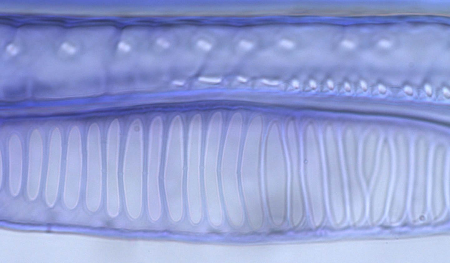
Vessel lengths
We often have to measure vessel lengths, a difficult task. Over the years we have refined the technique to where it is now as painless as possible. Stems or roots, or whatever is to be measured are cut, flushed (to refill any embolized vessels), and injected at about 30 kPa with a silicone-hardener mix (RTV-141 parts A & B, 10:1 A:B, Rhodia, Cranbury, NJ). We add 1 drop of 1% (w/w) uvitex optical brightener (Ciba Uvitex OB, Ciba Specialty Chemicals, Tarrytown, NY) in chloroform per gram of silicone, which makes the silicone easily visible under an epiflourescence microscope. It's important to avoid evaporation of the chloroform and precipitation of the uvitex. The injected silicone mixture should be clear. If it's cloudy, then crystals have precipitated. The silicone mixture does not penetrate typical pit membranes, and so it fills only the vessels cut open at the injection site. We inject overnight, remove stems and let the silicone set up for a few days. We then section the stem at ca. 6 distances starting near the injection site (between 3 and 10 mm) and ending where there are only a few filled vessels evident, which varies widely between species. The intervening distances are calculated from a logarithmic formula which concentrates the distances near the injection site where most of the vessels are (Christman et al. 2009, PDF).
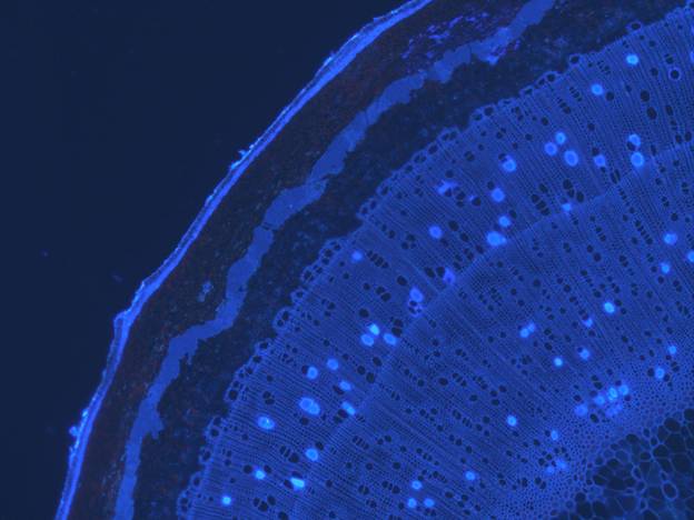
Vessels filled with the silicone + uvitex mixture are readily visible with fluorescence microscopy.
Photo: Frederic Lens
The number of filled vessels per xylem area are counted at each distance, and expressed as a percentage of the total vessels per xylem area at the injection point. Someday soon, in collaboration with Chuck Price (Georgia Tech), we hope to have an image-analysis program that semi-automates this tedious chore. A Weibull function is fit to the percentage of filled vessels vs. distance from injection. This function is used to derive the continuous vessel length distribution for the vessels at the site of injection. The principles and mathematics of this analysis are most accurately described in Christman et al. (2009, PDF). We have written two excel macros to do the computations. The first one fits the vessel data with the Weibull function ("fitlengthwiebull.xls"), and the second takes this Weibull function and calculates the vessel length distribution ("vesselengthprogramweibull3.xls").
Soil-Plant Water Transport Model
A version of this model (Sperry et al. 1998, PDF) is available for downloading, along with instructions for its use. Sorry it is so crude, I've always wanted to get back to this and revise it, and perhaps that will happen eventually. But for now, the program as is can be downloaded (HERE), with a guide.
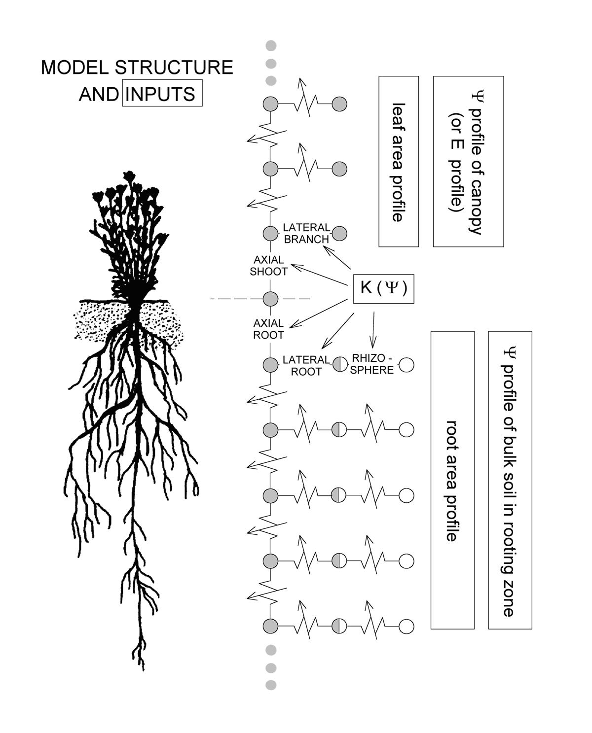
Model structure. See model instructions for full explanation.
Supply-Demand Hydraulic Model
Ecosystem models have difficulty predicting plant drought responses, partially from uncertainty in the stomatal response to water deficits in soil and atmosphere. We have developed a ‘supply–demand’ theory for water-limited stomatal behavior that avoids the typical scaffold of empirical response functions (Sperry and Love 2015, PDF; Sperry et al. 2016, PDF). The premise is that canopy water demand is regulated in proportion to threat to supply posed by xylem cavitation and soil drying. This theory has been implemented in a trait-based soil–plant–atmosphere model. The model predicts canopy transpiration (E), canopy diffusive conductance (G), and canopy xylem pressure (Pcanopy) from soil water potential (Psoil) and vapor pressure deficit (D). The Excel file containing the supply-demand hydraulic model described in Sperry et al. (2016) can be downloaded HERE. This file also includes a spreadsheet with instructions and an example on how to run the model.
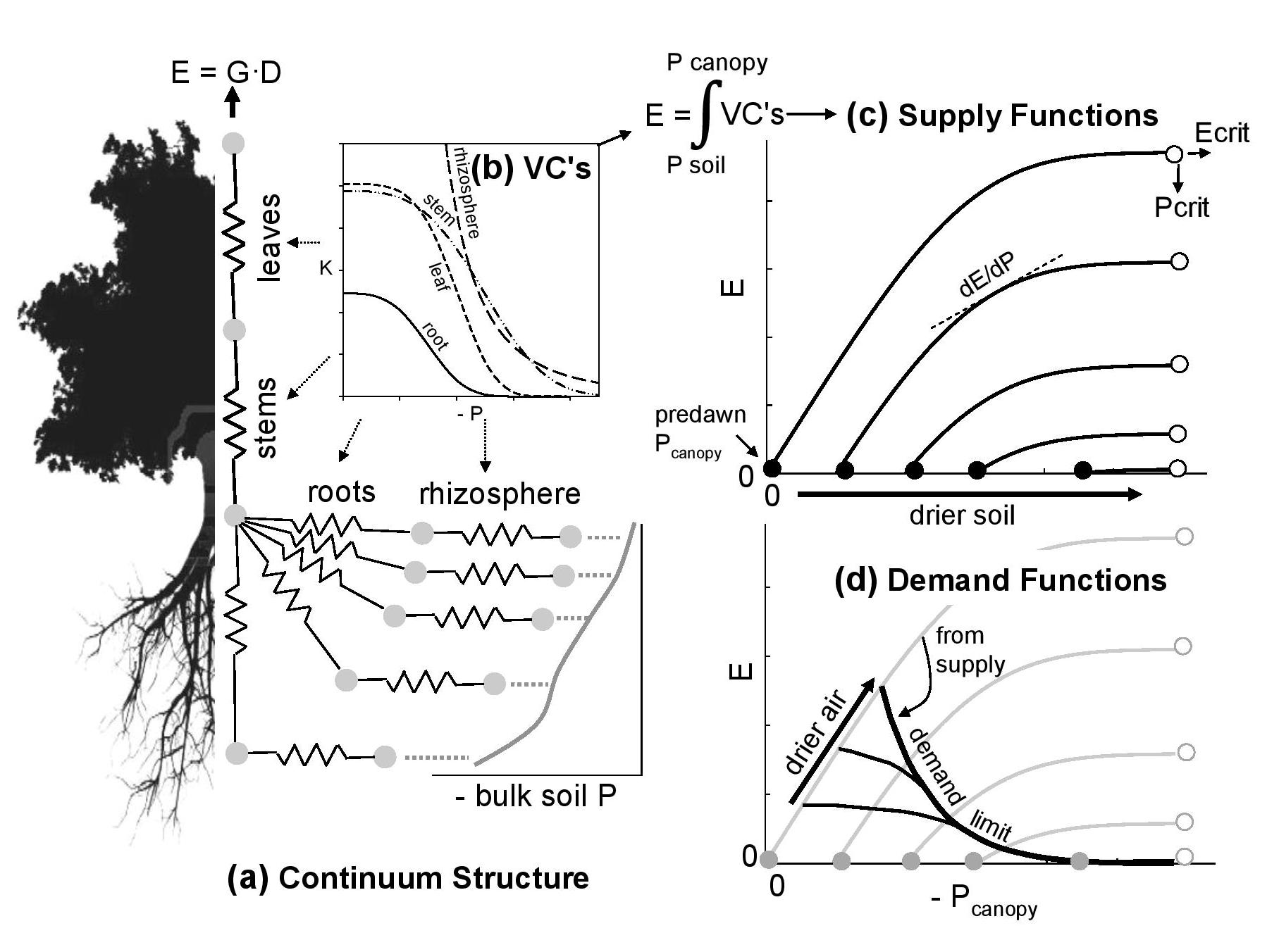
The supply-demand model. See Sperry et al. (2016) for full explanation.
Photosynthetic Gain And Hydraulic Cost Optimization Model
Existing land surface models struggle to represent the complex and species-specific stomatal responses to environmental conditions, especially soil drought. Currently we are working on developing a model that offers a solution to this problem by assuming that stomatal regulation aims to maximize photosynthetic gain minus hydraulic cost. Using the “Supply-Demand Hydraulic Model” as the foundation for the cost function we are building a trait- and process-based "profit-maximizing" algorithm which predicts realistic stomatal behavior in response to different environmental stimuli. The rationale of this modeling approach and an initial exploration of the model’s behavior are described in Sperry et al. (2017) [PDF]. This new approach to stomatal optimization theory may prove useful in large-scale modeling of responses to climate change.
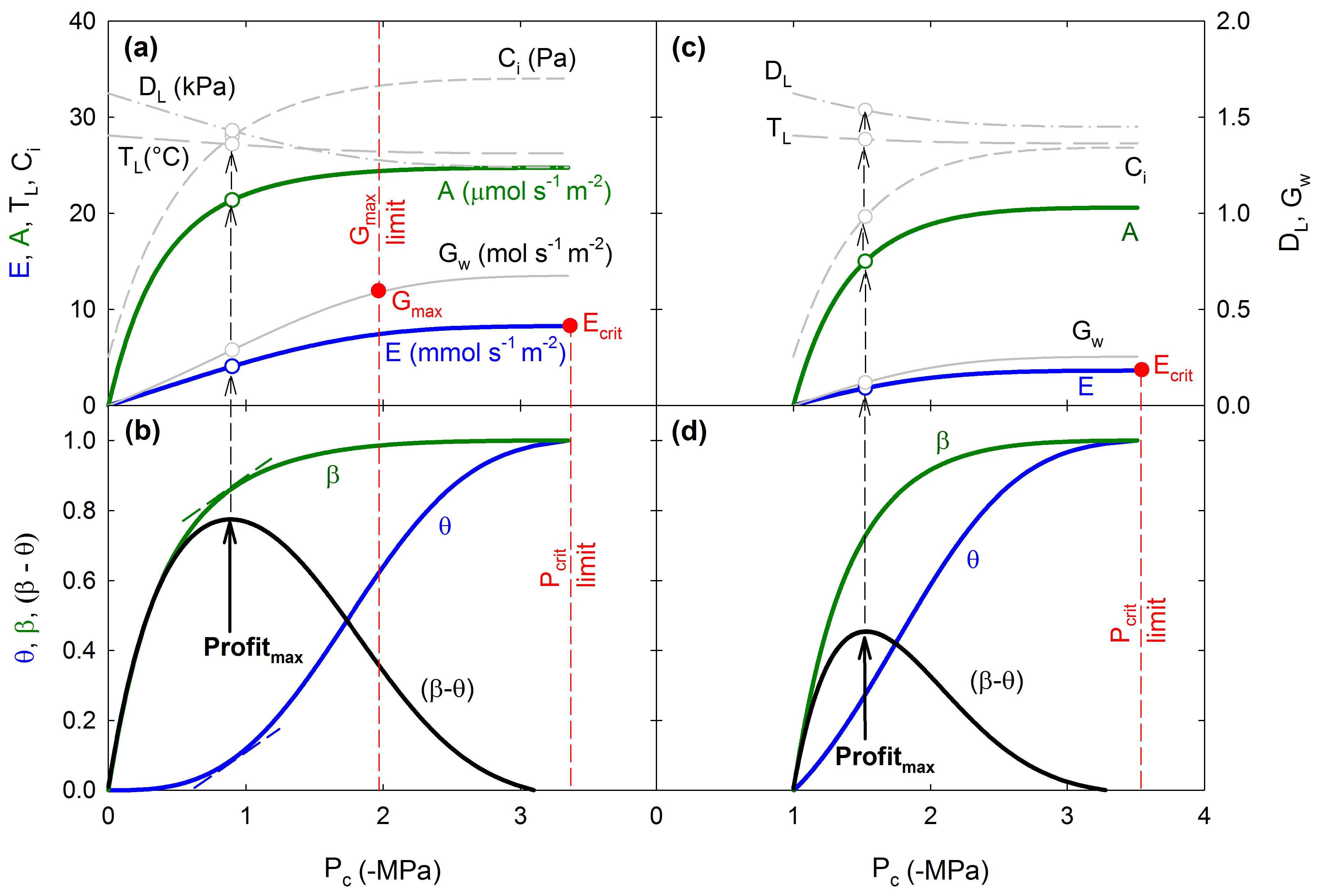
Photosynthetic gain and hydraulic cost optimization model. See Sperry et al. 2017 for full explanation.